Oct 12, 2026 · @KPM

Why one curve decides whether your relay trips

A cable fault on an 11 kV feeder pushes 8,000 A through a 400/1 A CT. That is 20 times its rating. The relay settings are right, and the CT passed its ratio test at commissioning. Yet the relay trips late, or a differential relay sees a "difference" that isn't really there.

The usual culprit is CT saturation. At normal load the CT copied the current perfectly. At fault current, with the wiring and relays actually connected to it, it could not.

The 5% and 10% error curves on a CT analyzer show exactly where that limit lies, for your CT and your wiring, in a single graph. This blog explains what the curves mean and how to use them on site, in plain language.

Where does a CT's error come from?

A CT never delivers 100% of the primary current to the relay. A small part is always used up inside the CT to magnetise its iron core.

•      Ip ÷ n is what the relay should see: the primary current divided by the CT ratio.

•      Ie (magnetising current) is the share the core keeps for itself. This is the error.

•      I2 is what the relay actually sees, after flowing through the CT's own winding resistance (Rct) and the connected burden (ZL).

So the error is simply:

\text{Error} = \frac{I_e}{I_p / n}

In a healthy, unsaturated core, Ie is tiny and the error is well under 1%. When the core saturates, Ie shoots up and the relay sees far less current than really flows in the fault.

Two things push a CT into saturation

To drive current through the relay and wiring, the CT must produce a voltage on its secondary side:

V = I_2 \times (R_{ct} + Z_L)

Every core has a ceiling for that voltage, called the knee point. Below it, the CT copies the primary current faithfully. Above it, a small extra voltage needs a huge magnetising current, and the error jumps.

Only two things raise that voltage:

1.     A bigger fault current. More current flows through the secondary.

2.     More burden. Longer cable runs, thinner cables, extra relays, meters and transducers on the same core.

This is the whole idea behind the error curve. If the fault current goes up, the burden must come down to keep the error in limit, and vice versa.

The 5% and 10% error curves, explained

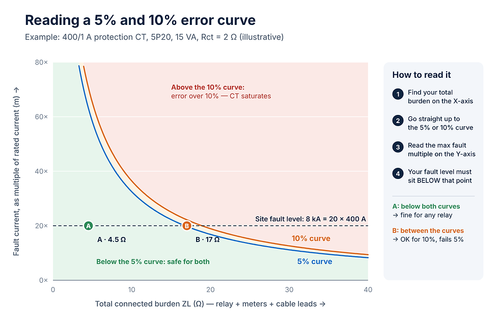
An error curve is a line of "limit points" for one CT. Each point answers one question: with this much burden connected, how big a fault can the CT carry before its error crosses 5% (or 10%)?

•      X-axis: total connected burden ZL, in ohms (relay + meters + cable leads).

•      Y-axis: fault current as a multiple of rated current, m (for example, 20 × 400 A = 8 kA).

•      Below the curve: error stays within the limit. Safe.

•      Above the curve: error exceeds the limit. The CT is saturating.

The 5% curve always sits just below the 10% curve, because a tighter limit allows less.

Example (illustrative CT: 400/1 A, 5P20, 15 VA, Rct = 2 Ω). The site fault level is 8 kA, which is 20 times rated current.

•      Point A, 4.5 Ω: a numerical relay and a short, healthy cable run. The 5% curve allows about 63 × here, so 20 × has a large margin. Fine for any relay.

•      Point B, 17 Ω: an old electromechanical relay, a panel meter and about 500 m of 2.5 mm² cable on the same core. The 5% curve allows only about 19.7 ×, so the CT just misses 5%. The 10% curve still allows about 22 ×, so it passes 10%.

Same CT, same fault, two different answers. The wiring decided it.

5% or 10%: which one does your relay need?

The nameplate already tells you which curve to check. In 5P20, "5" is the error limit in percent, "P" means protection class, and "20" is the accuracy limit factor (ALF): the CT holds 5% error up to 20 times rated current, at rated burden.

Always follow the relay manufacturer's CT requirement. High-impedance differential and REF schemes use Class PX CTs, which are specified by knee point rather than by these curves.

Practical relevance on site: 7 situations where the curve earns its keep

1.     The nameplate is a promise only at rated burden. "5P20, 15 VA" says nothing about your panel. The error curve shows the real accuracy limit at the burden actually connected.

2.     Cable leads can eat the whole margin, especially on 5 A CTs. 2.5 mm² copper is about 7.4 Ω per km. A 200 m run is a 400 m loop, about 3 Ω. On a 1 A CT that is 3 VA. On a 5 A CT it is 75 VA, five times a typical 15 VA rating.

3.     Adding a meter or relay to an existing core. Every new device adds burden. Read the curve first and see whether you are still below it at the site fault level.

4.     Relay retrofits. Replacing electromechanical relays with numerical ones cuts burden sharply. The curve shows how much margin you gain, or confirms an old CT can stay in service.

5.     Rising fault levels. A new transformer, a stronger grid connection or added generation raises fault current. Recalculate the fault multiple and check it against the curve.

6.     Investigating a mal-trip or a failure to trip. If the operating point sits above the curve, CT saturation is a likely contributor. That turns a guess into evidence.

7.     Accepting new CTs from a supplier. Measure the CT, plot the curve and confirm the class on the nameplate before it goes into the panel.

How a CT analyzer draws the curves without 8,000A

Nobody can inject 8 kA into a CT in a live switchyard. A CT analyzer does not need to. It measures the CT at low, safe levels and calculates how it will behave at fault current.

1.     Measure: ratio and polarity, winding resistance (Rct), and the excitation curve with its knee point.

2.     Calculate: build a model of the CT from that data, and work out the error at any fault current and any burden.

3.     Plot and judge: draw the 5% and 10% error curves, and check them against your site fault level and actual burden.

A few minutes with a portable kit tells you how the CT will behave during a real fault.

The KPM CT PT Analyzer

The KPM CT PT Analyzer runs this whole process in one connection and plots the error curves for protection CTs automatically.

•      Error curves for protection CTs: 5% and 10% curves from measured data, ready to compare against your site burden and fault level.

•      Low-frequency excitation testing: reaches the high knee points of EHV protection CTs with a low-voltage source, so the kit stays portable.

•      Complete CT picture in one run: ratio, phase and polarity, winding resistance, burden and excitation curve.

•      Auto nameplate deduction: works out an unknown CT's ratio, rated secondary and accuracy class when the nameplate is missing or unreadable.

•      Multi-tap testing: checks all secondary ratios of a multi-ratio CT in one operation.

•      Standards: complies with IEC 61869, and still supports IEC 60044 references found on older specifications and nameplates.

•      Built for the field: used in 220 kV, 400 kV and 765 kV live switchyards, as well as labs and CT manufacturing.

Behind every instrument is KPM's application support. Our engineers help your team set up the test, read the curves and decide what to do when a CT falls short.

Before you sign off a protection CT

•      Note the CT class on the nameplate (5P or 10P) and what the relay maker requires.

•      Find the maximum fault current at that location and divide by the CT primary rating to get m.

•      Add up the real burden: relay, meters, transducers and the cable loop resistance.

•      Read the 5% or 10% curve at that burden.

•      Confirm the fault multiple sits below the curve, with some margin.

•      If it does not: shorten or thicken the leads, move a meter to another core, or choose a CT with a higher ALF or knee point.

Quick FAQ

Is a CT that passes the ratio test good enough for protection? Not necessarily. A ratio test runs at normal current. The error curve tells you how the CT behaves at fault current, which is when protection actually works.

Can a 10P CT be used where 5P is specified? Only if the relay maker allows it. The 10P limit is loose, so the relay may see a less accurate fault current.

Why does my CT pass in the lab but fail on site? The lab usually tests at rated burden. On site, long cable runs and extra devices add burden and push the operating point above the curve.

Do I need to inject full fault current to plot the curves? No. A CT analyzer calculates them from low-level measurements of ratio,